Loan App Prediction using machine learning in Python
How to be a smart shylock

Angela has some disposable income that she wants to invest in a money lending business. This kind of business has several risk factors associated with it. How can Angela make data driven decisions on whom to lend money to?
Expectations
The end goal is to make this a binary classification problem where given a set of inputs, the model either gives a prediction of approved or rejected. The approved prediction means Angela can go ahead and give the loan to the applicant while rejection means Angela will either have to revisit the decision manually or outright trust the model.
Loading the Data
For this problem, we will be using the data set on loan prediction on Kaggle. You can download the data from here
You will need to use scikit-learn version 0.23.2 for the project to run smoothly
pip install -U scikit-learn==0.23.2
Import the relevant libraries needed ```py
Importing important libraries
import pandas as pd import numpy as np import matplotlib.pyplot as plt import seaborn as sns import plotly import plotly.express as px import plotly.figure_factory as ff from sklearn.utils import resample from sklearn.preprocessing import StandardScaler , MinMaxScaler from collections import Counter from scipy import stats
Classifiers
from sklearn.ensemble import AdaBoostClassifier , GradientBoostingClassifier , VotingClassifier , RandomForestClassifier from sklearn.linear_model import LogisticRegression , RidgeClassifier from sklearn.discriminant_analysis import LinearDiscriminantAnalysis from sklearn.model_selection import RepeatedStratifiedKFold from sklearn.neighbors import KNeighborsClassifier from sklearn.model_selection import GridSearchCV from sklearn.tree import DecisionTreeClassifier
from sklearn import tree from sklearn.naive_bayes import GaussianNB from xgboost import plot_importance from xgboost import XGBClassifier from sklearn.svm import SVC
#Model evaluation tools from sklearn.metrics import classification_report , accuracy_score , confusion_matrix from sklearn.metrics import accuracy_score,f1_score from sklearn.model_selection import cross_val_score
#Data processing functions from sklearn.preprocessing import StandardScaler from sklearn.model_selection import train_test_split from sklearn import model_selection from sklearn.preprocessing import LabelEncoder le = LabelEncoder()
Load the data from the csv. Replace ”./path to csv” with where your data is located.

```py
    data = pd.read_csv("./path to csv")
We load the dataset as a pandas dataframe and store it in data. We can view our data as follows py data.head(4)
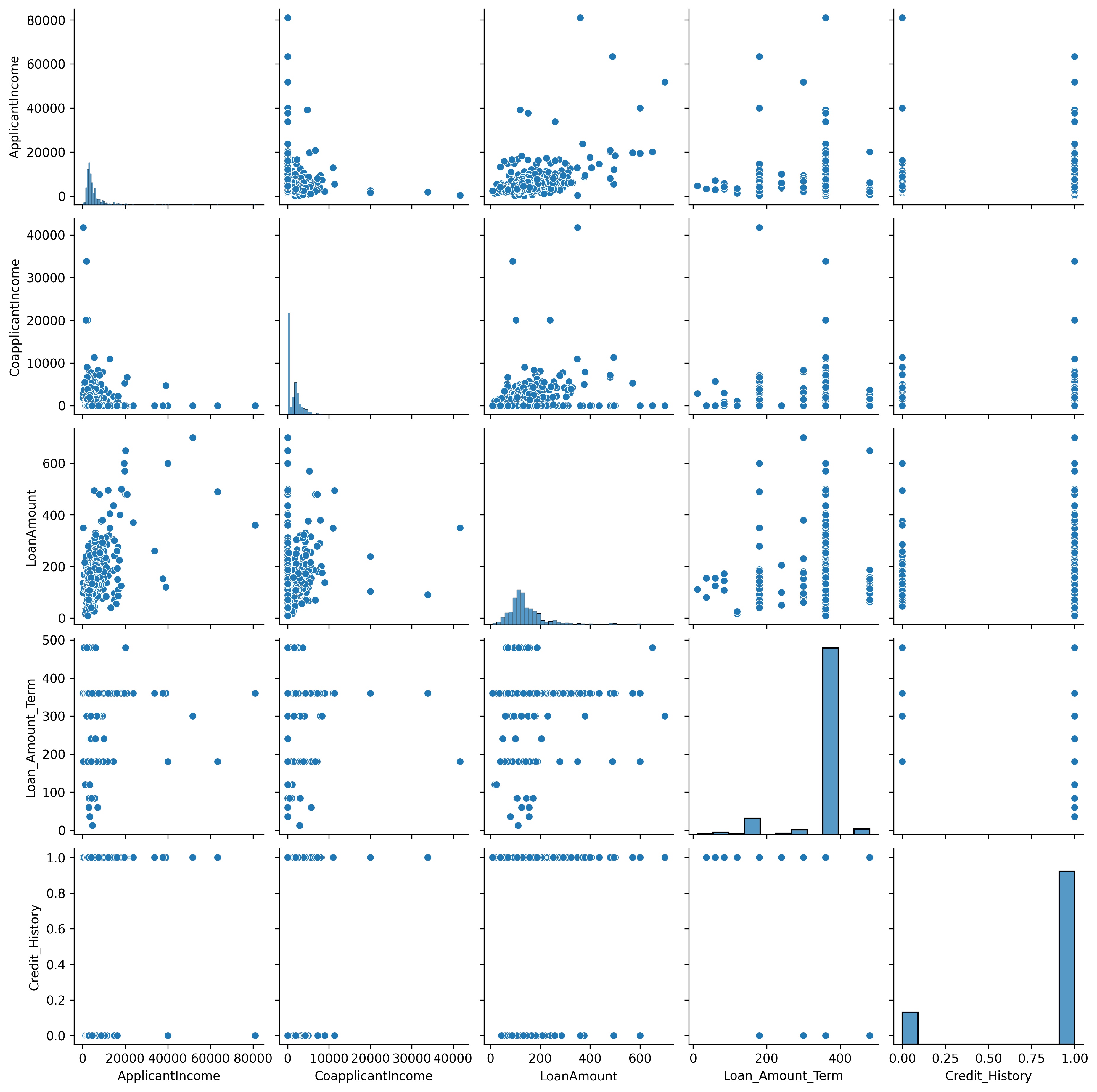
Exploratory data analysis We first draw a scatter plot of all variables against themselves in a bivariate fashion. py sns.pairplot(data) plt.show()
data.describe()
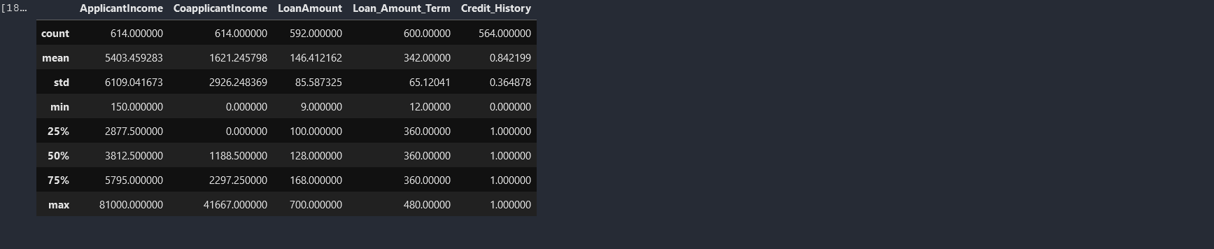
From the above results from the describe function, we can see that some columns have missing values as indicated by the count. The standard deviation(std) also tells us more on how the data is distributed. Low standard deviation means data points are clustered around the mean, and high standard deviation indicates data is more spread out. We might need to investigate further on the data points on the ApplicantIncome and CoapplicantIncome columns as the std is too high which might indicate presence of outliers. Before we can do any manipulations we need to understand our column datatype using the info() function. py data.info()
We have a dataset with 4 distinct datatype. The Loan_ID column does not help with our predictions, so we drop it. You will not qualify for a loan just because your loan id is a certain value.
data = data.drop(["Loan_ID"],axis=1)
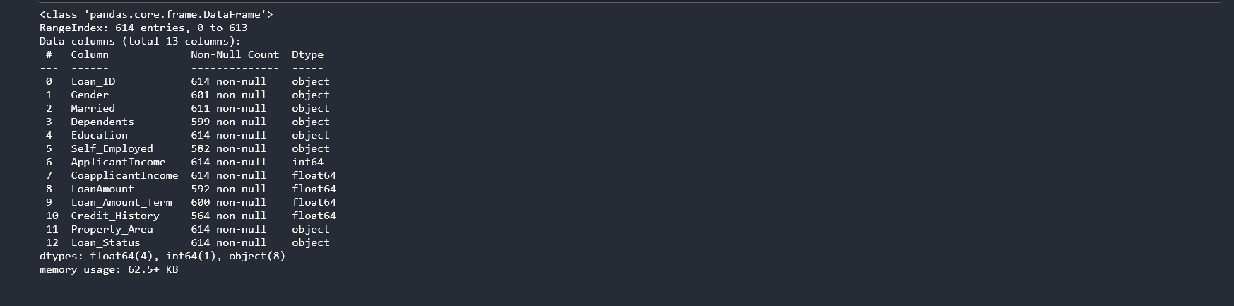
Are graduates more eligible for loans than non-graduands?
                sns.catplot(x='Loan_Status',
                            y='LoanAmount',
                            hue="Education",
                            ci="sd",
                            palette="dark",
                            alpha=.6,
                            height=6,
                            data=data,
                            kind='bar',
                           );
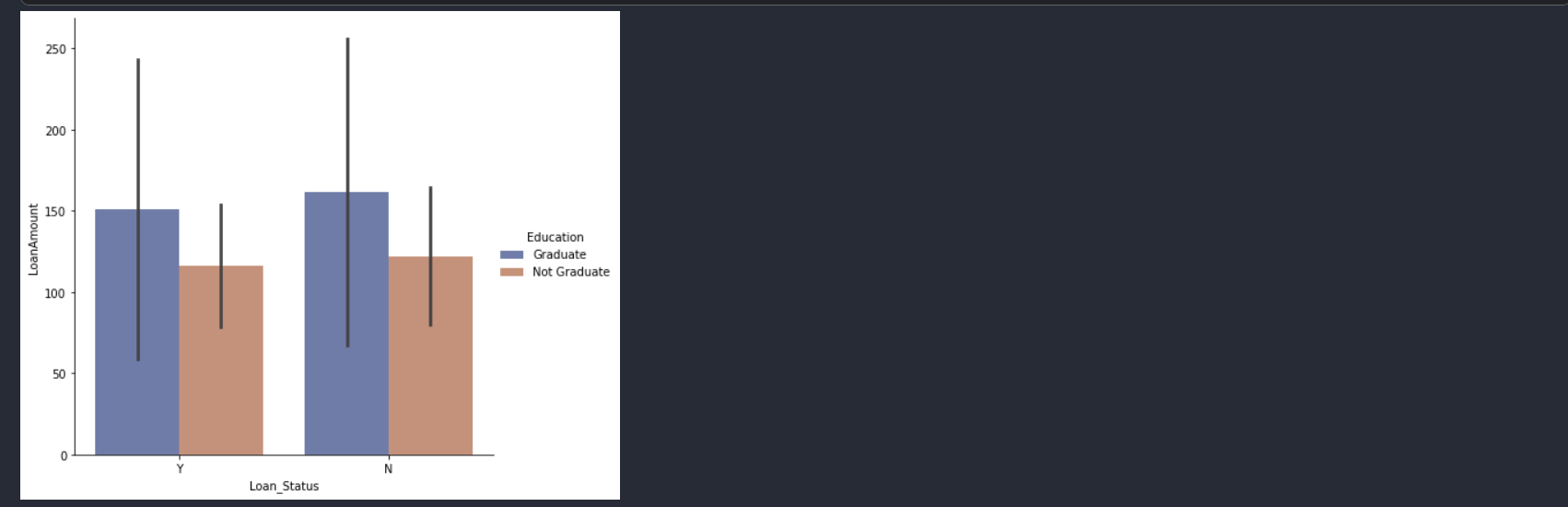
Are women more likely to get loans than men?
  sns.catplot(x='Loan_Status',
                            y='LoanAmount',
                            hue="Gender",
                            ci="sd",
                            palette="dark",
                            alpha=.6,
                            height=6,
                            data=data,
                            kind='bar',
                    );
Are single people more likely to get loans than married people? ```py sns.catplot(x='Loan_Status', y='LoanAmount', hue="Married", ci="sd", palette="dark", alpha=.6, height=6, data=data, kind='bar', );

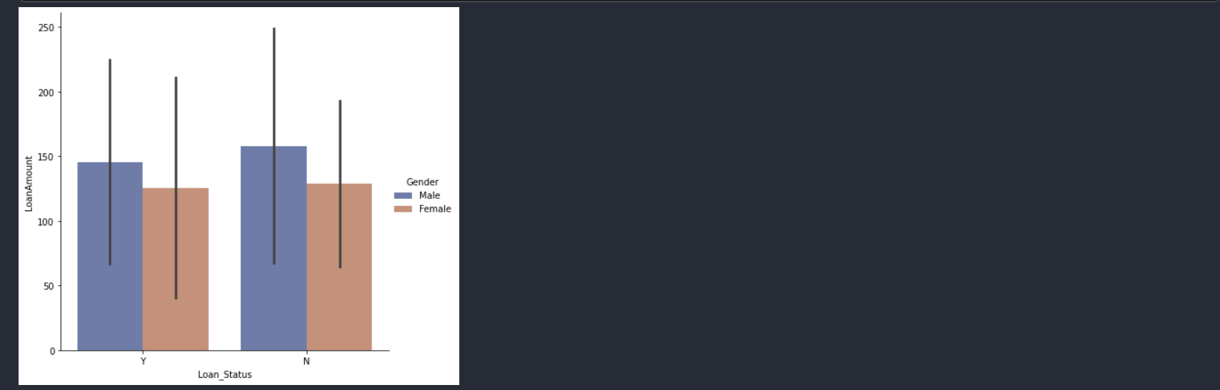
From the std, we suspect having outliers in the Applicant Income and coapplicant income. Lets start by first visualizing the distribution of the data in the ApplicantIncome to verify that we indeed have outliers that are accounting for the high std.
```py
fig = px.scatter_matrix(data["ApplicantIncome"])
fig.update_layout(width=700,height=400)
fig.show()
The ApplicantIncome scatter plot visually confirms that the column has outliers. Next we work on the visualization of the CoapplicantIncome column.
fig = px.scatter_matrix(data["CoapplicantIncome"])
fig.update_layout(width=700,height=400)
fig.show()
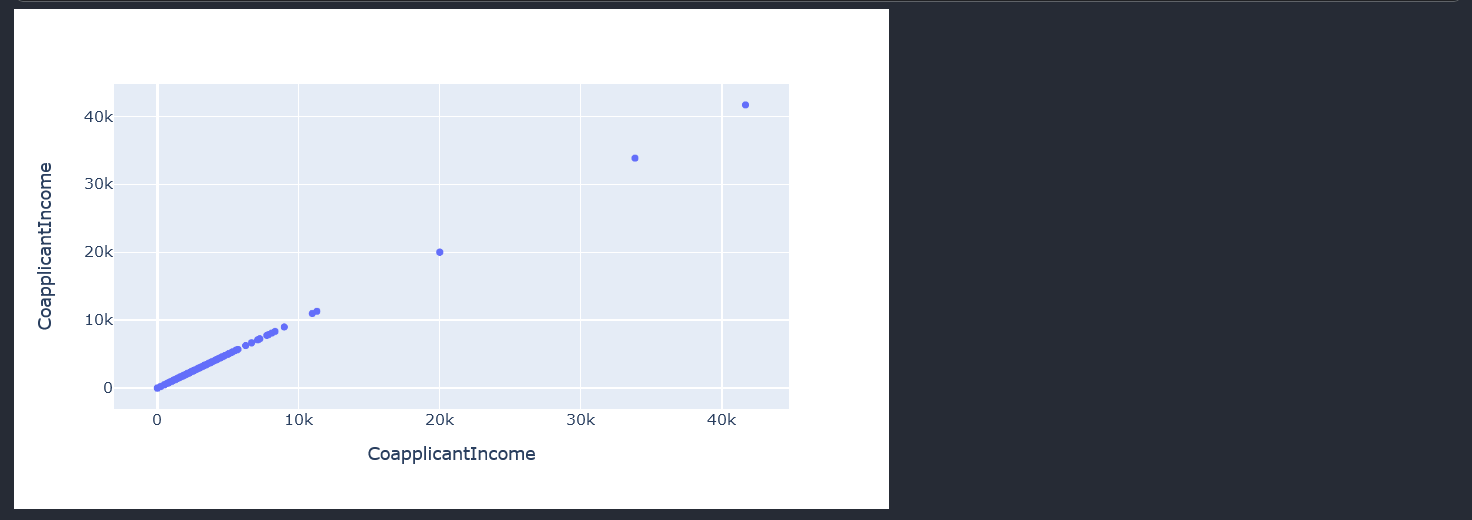
As expected, the visual plot of the Coapplicantincome also shows our outliers.
To make work easier as the notebook grows, I will be writing all our model predictions on an external txt
import os
if os.path.exists("results.txt"):
   os.remove("results.txt")
else:
   print("The file does not exist")
def write_results_to_file(txt):

  f = open("results.txt","a")
  f.write(txt + '\n')
  f.close()

def print_line(name):
    write_results_to_file(f'------------------------------------------------------------{name}----------------------------------')
    print(f'------------------------------------------------------------{name}----------------------------------')
The above code just removes any old files named results.txt on our file system and creates one if it does not exist. The write_results_to_file appends a new line to the results.txt while the print_line adds a divider to the write_results_to_file file. Checking the distribution of the data
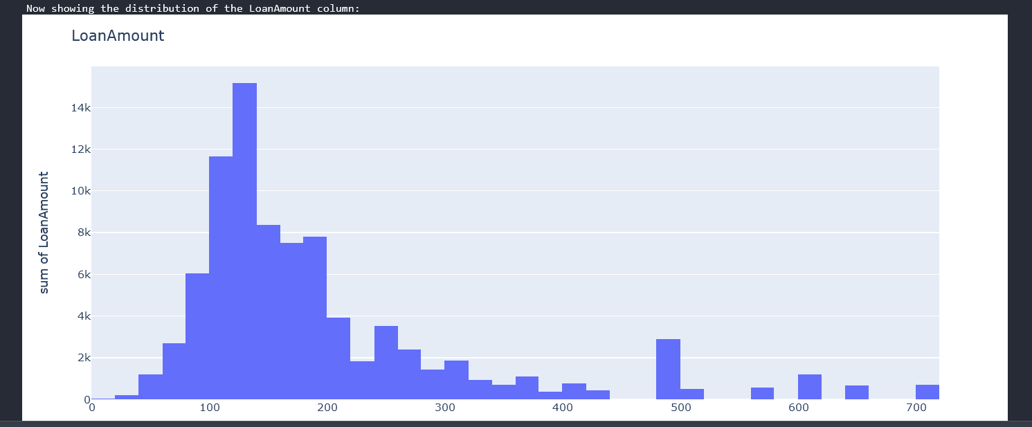
Ideally,to get the best possible results our data needs to be in a normal distribution. Data in a normal distribution observes the bell curve.
def check_distribution_of_column(column_name):
  fig = px.histogram(data[column_name],x =column_name,y = column_name)
  fig.update_layout(title=column_name)
  fig.show()
The function check_distribution_of_column takes in a column name and plots a histogram showing the distribution of data in that column. We iterate through all the columns in our data-frame calling on our handy function to draw the distribution.
for col in data.columns:
    print("Now showing the distribution of the " + col + " column:")
    check_distribution_of_column(col)
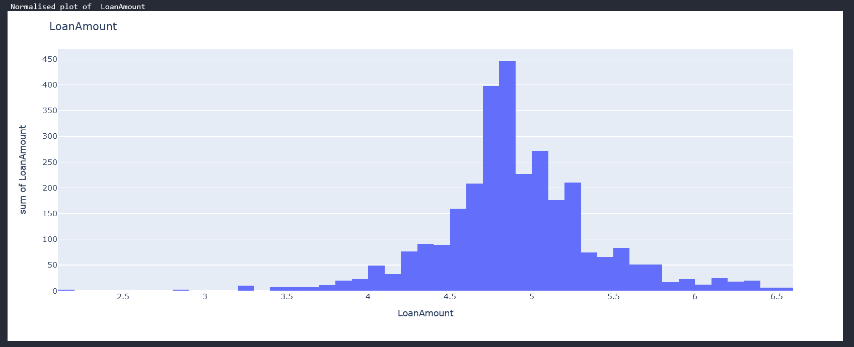
You should be having individual plots of each column. The loan amount plot looks like this
From the above graphs we can see that we have a mix of categorical variables and discrete variables. Categorical variables contain a finite number of categories or distinct groups. Categorical data might not have a logical order. For example, categorical predictors for our data-set are gender,marital status,self employed etc. Discrete variables are numeric variables that have a countable number of values between any two values for example the applicants income, coapplicantincome and loan amount. With all these, we can now begin some data cleaning.
Data Cleaning
From our EDA we have established we have some problems we need to fix with the data :
Deal with null values to ensure our data is of same length Deal with outliers Find a way of converting categorical variables to discrete variables since our model will expect to use discrete values. Find a way to make the data normally distributed
- Dealing with null values We have a few options:
Drop all rows with at least one null value Replace the null value with either the mode, mean or median of the column. For the first approach, we do not have much data to work with as such I will be exploring the second option. Also dropping the null values doesnt necessarily mean that we will not be dropping more rows as we continue with the data cleaning. We might need to drop more rows in future and thus greatly reduce our dataset. Option 2 is our best bet.
# shows number of missing values by column
data.isnull().sum()
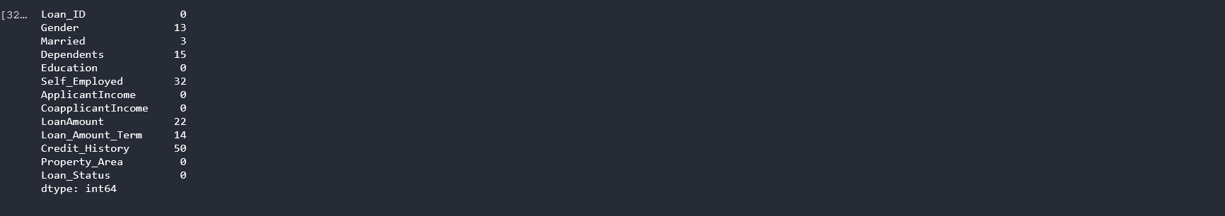
For the categorical variables, I will use the mode of the column. For example, we have more men in the dataset so the probability of someone with a null value having being a man was higher than it being a woman.
data["Gender"].fillna(data["Gender"].mode()[0],inplace=True)
data["Married"].fillna(data["Married"].mode()[0],inplace=True)
data["Self_Employed"].fillna(data["Self_Employed"].mode()[0],inplace=True)
data["Loan_Amount_Term"].fillna(data["Loan_Amount_Term"].mode()[0],inplace=True)
data["Dependents"].fillna(data["Dependents"].mode()[0],inplace=True)
data["Credit_History"].fillna(data["Credit_History"].mode()[0],inplace=True)
# shows number of missing values by column
data.isnull().sum()
Now checking for null values, we notice only the LoanAmount still has nulls which is a discrete variable.To fix this we will use the median since we had already established an outlier for this column. Thus using the mean might not give an accurate representation of roughly how much might have been borrowed.
data["LoanAmount"].fillna(data["LoanAmount"].median(),inplace=True)
All done with dealing with null values.
2. Dealing with outliers We have three discrete variables of which two have outliers. py data["ApplicantIncome"] = np.log(data["ApplicantIncome"]) #As "CoapplicantIncome" columns has some "0" values we will get log values except "0" since log 0 is undefined data["CoapplicantIncome"] = [np.log(i) if i!=0 else 0 for i in data["CoapplicantIncome"]] data["LoanAmount"] = np.log(data["LoanAmount"]) We apply the natural logarithm to all our discrete variables to normalize the data. Natural log transformations reduce skewness to our datasets. Compare our loan amount distribution now with what we had above.